content type highlightpublished December 7, 2021
Interpretable Adaptive Optimization
Interpretable Adaptive Optimization
Providing new features—while preserving user privacy—requires techniques for learning from private and anonymized user feedback. To learn quickly and accurately, we develop and employ statistical learning algorithms that help us overcome multiple challenges that arise from sampling noise, applications of differential privacy, and delays that may be present in the data. These algorithms enable teams at Apple to measure and understand which user experiences are the best. This understanding leads to continual improvements across Apple’s products and services to drive better experiences. We provide aspects of this understanding to the Apple developer community through features such as product page optimization.
The algorithmic solution used in product page optimization is discussed in detail in our paper, Smooth Sequential Optimization, which was recently accepted at the workshop on Bayesian Causal Inference for Real World Interactive Systems at the KDD 2021 conference. In this post, we take you through how we apply robust Bayesian inference to generate interpretable knowledge by learning sequentially from realistic user behavior. As we show, Bayesian methods can be extended further. Using reinforcement learning we can learn from user feedback and adapt to identify the optimal user experience, while carefully balancing the speed of adaptation against algorithmic stability and interpretability.
To understand the kinds of problems we work on, let’s start with a simple example. In the recently released product page optimization feature on the App Store, developers can learn about which variation of their app icon is the most appealing and engaging to users, and hence which one drives more downloads to their app, as seen in Figure 1. A well-known approach to generate such learnings is to run a randomized controlled experiment in which we randomly show a subset of visitors one of the two alternatives, also called variants. This is followed by a hypothesis test to estimate the statistical confidence that variants differ from each other, based on the private and aggregated responses relating to each. We use this specific methodology in product page optimization.

A complementary perspective comes from research into the multi-armed bandit problem, a simple form of reinforcement learning that aims to adapt the selection of alternatives, over time, to maximize long-term value, or yield. While both approaches—randomized control trials and multi-armed bandits—have received attention in academia and industry, they tend to be seen as separate topics. But for a majority of our work, we consider an intermediate perspective.
Within this complementary perspective, hypothesis testing can be seen as a formalized method where a human operator first learns about the relative values of a set of variants, and then takes some action based on this knowledge to help meet their objectives. Bandit-based reinforcement learning automates this process, employing an algorithm to perform some decisions on behalf of the human operator.
Why do we want to achieve this confluence between hypothesis testing and multi-armed bandits? To facilitate optimization with humans in the loop. Human operators are often involved in applying optimization in industry. These experts are involved in business-relevant interpretation, higher-order decision-making and meta learning about what delivers value in the long run. For example, human operators might want to use hypothesis testing, based on the knowledge accrued so far, to add or remove treatments during an ongoing optimization process. Hence, finding a sweet spot between experimentation and optimization can enable human operators to generate meaningful interpretations backed by sound statistical evidence, while also maximizing yield.
One especially important challenge we face when learning sequentially about the value of different treatments is that of delayed data. When we lean toward yield maximization through dynamic traffic allocation, the impact of delayed data is more pronounced. If we wait until all delayed feedback is received, the learning algorithm, or agent, cannot update its knowledge in the interim, potentially losing yield. So we’d like to find a way to update the agent at a cadence that we control, decoupling updates from the structure of the delay. One approach is to assume that at each update, the agent receives only partial feedback—a composite of responses generated by assignments at some point in the past. Note that our composite feedback is anonymous: Not only is our data privately aggregated; we are even precluded from knowing which specific batch of past assignments generated a response. All we know is that we have a number of responses, and each is delayed by a potentially different amount of time.
Delayed feedback causes some problems for our agent when it wants to update its knowledge about the relative value, or rewards, of the treatments. If we use standard maximum likelihood estimation (MLE) to estimate treatment rewards, we often observe unstable oscillatory dynamics. This instability makes human-in-the-loop decision making challenging because what appear to be the better performing variants can change unpredictably.
We can demonstrate this issue with a simple example, as shown in Figure 2. We’ve simulated two treatments with a 5% stationary difference in true rewards, but with a delay generated by a Poisson distribution (with a lambda parameter of 5). If we simply assign the treatment that has the current best maximum likelihood of being the best one, the number of assignments per treatment oscillates around for a while as seen in Figure 2. The delays produce noise in the maximum likelihood estimates, which seesaws between overestimating and underestimating a treatment’s true reward. Things eventually resolve themselves under assumptions about stationary true rewards. As we show later, we also see ongoing instability if the true rewards themselves are changing, on top of delayed feedback. As a result, human operators would find it challenging to reliably interpret the relative performance of these treatments.
To better address the problem of estimating true value in the face of noise, we model treatment rewards using Bayesian inference. We calculate:
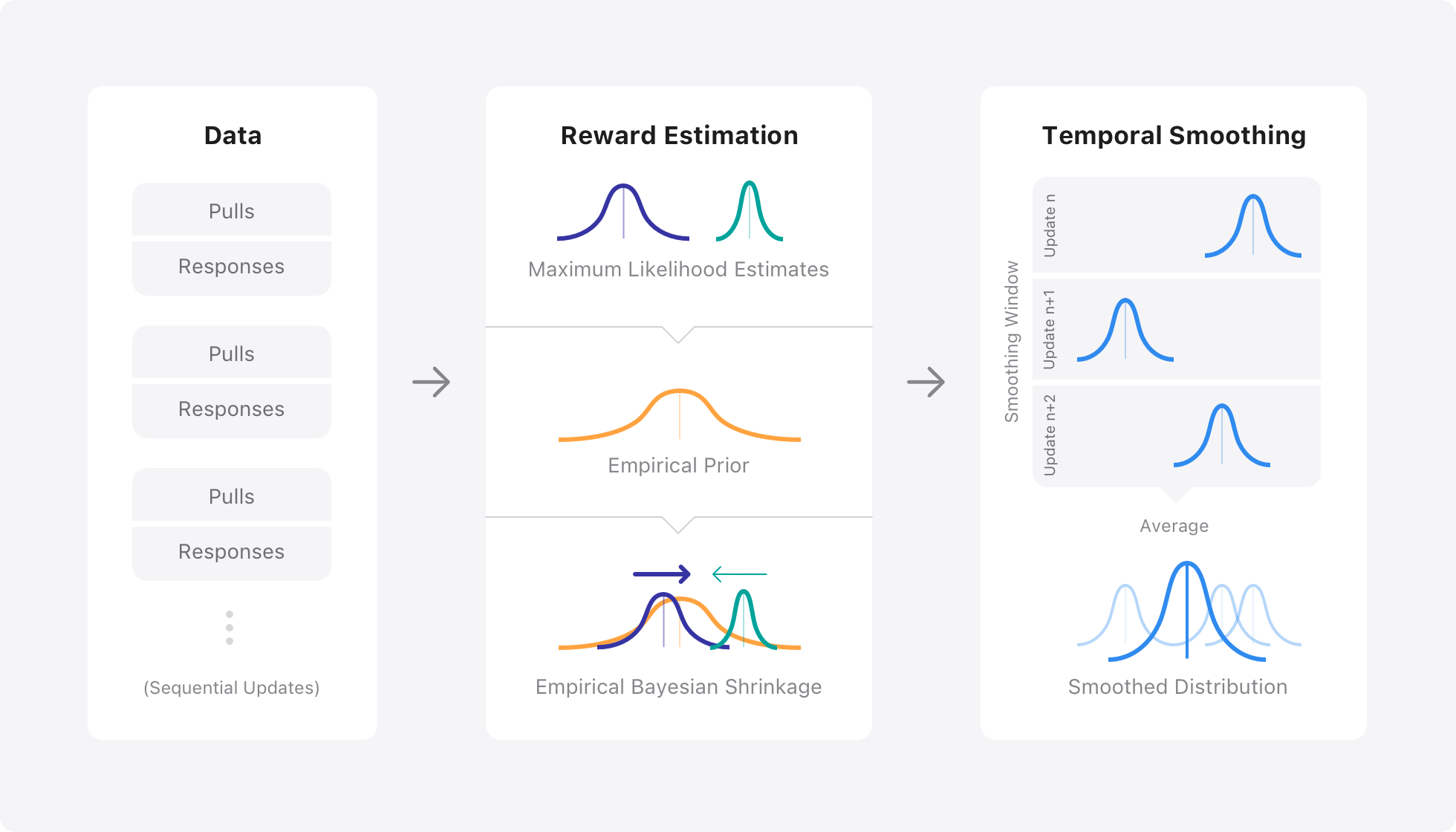
The more times a variant is tried out, the more we can learn about it and hence lower our uncertainty in its estimate. More specifically, we employ Empirical Bayesian shrinkage estimation as an alternative to maximum likelihood to estimate rewards during sequential hypothesis testing. Additionally, when adapting traffic with a Thompson sampling bandit, we apply windowed temporal smoothing, as shown in Figure 3.
The rationale for this approach is fourfold:
Let’s look at each of these rationales in detail.
First, empirical Bayesian inference acts as a form of regularization during reward estimation, modulating our knowledge based on the ratio of signal to noise in the data. We adapt previous work in this space to construct a prior distribution of treatment rewards from our observed data. This prior is then used to shrink the maximum likelihood estimates towards the prior mean. The more the uncertainty in the estimate, the more we shrink it towards the prior mean. For example, as shown in Figure 3, we’re more uncertain about the dark blue treatment’s true reward, hence we shrink it more towards the prior mean. This shrinkage is calculated using the James-Stein estimator.
Second, this empirical Bayesian approach allows us to trade precise estimation of individual rewards for learning about the relative value of different treatments. This is a pragmatic trade-off within an industry setting. We’re usually more interested in learning which treatment performs the best, and less in need of knowing the exact reward value of each variant. Moreover, this trade-off helps us to optimize in situations where we have tens or hundreds of treatments, and we want to quickly identify a subset of better-performing ones.
Developers that use product page optimization automatically benefit from both of these facets of Bayesian inference. Regularization ensures that developers are not presented with potentially incorrect estimates of conversion rates in high-noise scenarios, such as at the beginning of a test. And, by prioritizing learning about the relative value of different treatments, they can experiment on multiple variants of their product page without needing large traffic volumes to achieve meaningful results—as would be required by other standard techniques like Bonferroni correction.
Third, injections of differential privacy noise can adversely affect accurate reward estimation under MLE. As we strive to introduce stricter mechanisms to better protect user privacy, we need to employ more robust approaches to estimation. Noise-sensitive empirical Bayesian shrinkage helps us learn better in a private world. For the same user privacy, we achieve better understanding of aggregate performance.
Lastly, by applying windowed temporal smoothing to the empirical Bayesian estimates, we help address the fluctuating overestimation and underestimation of treatment rewards that delayed feedback causes as we shift traffic between treatments. In our current approach, we apply windowed temporal smoothing over past empirical Bayesian reward estimates as seen in Figure 3. We’ve evaluated a couple of different smoothing kernels that allow us to balance speed against stability of adaptation. Following the smoothing, we now have updated posterior reward distributions that we then use to assign treatments until the next update, using stochastic Thompson sampling.
The benefit of smoothed empirical Bayesian estimation can be seen by returning to our simple example above. Treatment assignments adapt to the best treatment in a more stable manner as shown in Figure 2. As is also evident in the figure, this adaptation is more gradual and interpretable. In large simulations involving multiple treatments and variable delays, we’ve confirmed that the value of our approach grows as the number of treatments increases. Other researchers have also found that empirical Bayesian estimation is great at weeding out poorly performing treatments and adapting with greater stability. It’s worth noting that these advantages come without losing much in terms of regret, which is initially higher but then becomes very similar to what maximum likelihood estimation can deliver in the longer term.
The reason that smooth empirical Bayesian inference delivers more stable performance is easy to understand when we look at reward estimation error over consecutive updates, as shown in Figure 4. Maximum likelihood estimation is noisier, especially early on, due to the over- and underflow in responses due to delayed feedback. However, with smooth empirical Bayes, we observe a more gradual and stable reduction in estimation error. This in turn helps ensure stable changes in treatment assignments over time.
Going back to our original goals, in addition to boosting yield we also want to want to facilitate sequential hypothesis testing and human interpretation. That is, we want to statistically compare the rewards of treatments at any point during the sequential learning process. This information could, for example, be used to conclude a test earlier if there are clear differences between variants, or to remove poorly performing treatments in a bandit.
We conduct sequential hypothesis testing using Bayes factors. Specifically, we entertain a pair of hypotheses:
We construct likelihood distributions of the true mean difference between the treatment rewards under both hypotheses. Given the estimated differences in rewards after applying smooth shrinkage, we calculate the Bayes factor as a likelihood ratio in terms of the relative likelihood of the observed difference under the likelihood distributions corresponding to the two hypotheses. We repeat this calculation at every update, enabling downstream inference based on interpreting these Bayes factors. Interpretation involves using one of the following two approaches:
Indeed, the confidence values shown to users of product page optimization are exactly the complement of these Bayesian false discovery rates.
We can compare the maximum likelihood and empirical Bayes approaches in terms of their ability to support hypothesis testing using Bayes factors. Over a large number of diverse simulations, we find that Bayesian inference yields higher Bayes factors earlier when there are real effects, and yields lower Bayes factors when no real effects exist.
More specifically, when applying MLE to the range of possible behaviors expected in product page optimization, we achieve a type I error of 38% over a 90-day period. But, when we instead use empirical Bayes, we see that this error reduces by a factor of more than 4. The combination of Bayesian inference and sequential hypothesis testing via Bayes factors ensures that product page optimization is robust and that its results are trustworthy.
We also apply sequential hypothesis testing alongside dynamic changes to traffic allocation using Thompson sampling. We find that smooth empirical Bayesian estimation produces higher Bayes factors earlier when there are real effects. Ultimately, this translates to an important advantage of using such Bayesian methods: increased statistical power for detecting true positives, and a lower type I error due to false positives, as shown in Figure 5. This effectively means more statistical confidence to underpin human-led decision-making, such as treatment addition and removal. The underlying reason behind this advantage is the fact that smooth empirical Bayesian reward estimation results in a better strategy for balancing exploration and exploitation early on.
Our smooth shrinkage algorithm becomes even more useful when the true rewards can change over time. The variability in true rewards can be arbitrarily complex and potentially intractable to solve in all cases. Furthermore, reliable hypothesis testing can be challenging under such circumstances. Generally speaking, accurate reward estimation can be challenging under various types of non-stationarity. For example, tracking symmetric variations in true rewards alongside changing traffic allocation can result in a temporal version of Simpson’s paradox. Additionally complicating the situation is noise introduced by delayed feedback, which adversely affects our ability to distinguish real change from apparent (noise induced) variation.
Maximum likelihood estimation is overly susceptible to the noise generated by the combination of delayed feedback and the change in true rewards. A negative feedback loop between the instability in estimation error and the failure to adapt to the best treatment results in poor performance.
To address the challenges posed by changing circumstances, we first compute estimates after grouping treatment responses by time of assignment. Then, when applying smooth empirical Bayesian shrinkage, we weight these estimates per update. This ensures that relative changes in true rewards can be better estimated, by providing more separation of symmetric changes over time. Finally, we employ empirical Bayesian estimation within a finite-length smoothing window, similar to the idea of discounted smoothing. As a smoothing window travels over changes in true rewards, it enables us to learn about the change. Smooth empirical Bayes estimation is much more stable in adapting to a change in true rewards, in spite of noise generated by delayed feedback, even if it is slightly slower to adapt. The trade-off between adaptation speed and stability is controlled by the size and shape of the smoothing kernel.
We’ve outlined a Bayesian approach that combines bandit-based optimization with interpretability, using sequential hypothesis testing. By introducing this we can begin to balance the learning-yield trade-off, maximising yield to some degree, while also providing interpretable learnings for human operators. Possible future extensions include continuous online learning where treatments can be added and removed at any point, transfer learning from previously conducted tests, factorial bandits using hierarchical Bayesian methods, and more.
We’ve adopted empirical Bayesian estimation as an algorithmic approach due to synergies with Bayesian sequential hypothesis testing. As we’ve shown, it can help alleviate the challenges inherent in adaptive optimization with delayed feedback. Not only can it help us stabilize adaptation; we can more robustly estimate value across a number of scenarios—including, but not limited to, situations in which differentially private noise is present. Further, this method improves the power of Bayesian hypothesis testing for higher-order decision making. Finally, in changeable real-world conditions, we can control the trade-off between the speed and stability of adaptation.
The algorithms we’ve discussed here help Apple’s developer community improve their product pages on the App Store. In product page optimization we strive to maximize learning and, hence, we do not adapt the rate at which we show each variant. Nonetheless, we still use empirical Bayesian estimation to enable developers to progressively learn about the relative performance of product page variants. This gives them results as soon as data is received. Developers can conclude testing as soon as they deem variants to show significantly different performance, with confidence that our approach avoids inflated risks of false positives.
We’d like to acknowledge the authors Srivas Chennu, Andrew Maher, and Jamie Martin as well as the valuable feedback and input from Puli Liyanagama, Phil Mohr, Aleks Iljina, Rajiv Krishnamurthy, Garrick McFarlane, Nick Kistner, Jae Hyeon Bae, and Nihar Hati.
Chennu et al., “Smooth Sequential Optimisation with Delayed Feedback”, Workshop on Bayesian Causal Inference in Real World Interactive Systems, KDD, 2021. [link].
Deng, Lu, and Chen, Continuous monitoring of A/B tests without pain: Optional stopping in Bayesian testing, DSAA, 2016. [link].
Dimmery et al., Shrinkage Estimators in Online Experiments, KDD, 2019. [link].
Garg and Akash, Stochastic Bandits with Delayed Composite Anonymous Feedback, arXiv, 2019. [link].
Jin and Pekelis, Acceleration of A/B/n Testing under time-varying signals, 2018. [link].
Kass and Raftery, Bayes Factors, Journal of the American Statistical Association, 1995. [link].
Gavrier and Moulines, On Upper-Confidence Bound Policies for Non-Stationary Bandit Problems, arXiv, 2008. [link].
Schönbrodt et al., Sequential Hypothesis Testing with Bayes Factors: Efficiently Testing Mean Differences, Psychological Methods, 2017. [link].
A Multi-Task Neural Architecture for On-Device Scene Analysis
June 7, 2022research area Computer Vision, research area Methods and Algorithms
Scene analysis is an integral core technology that powers many features and experiences in the Apple ecosystem. From visual content search to powerful memories marking special occasions in one’s life, outputs (or “signals”) produced by scene analysis are critical to how users interface with the photos on their devices. Deploying dedicated models for each of these individual features is inefficient as many of these models can benefit from sharing resources. We present how we developed Apple Neural Scene Analyzer (ANSA), a unified backbone to build and maintain scene analysis workflows in production. This was an important step towards enabling Apple to be among the first in the industry to deploy fully client-side scene analysis in 2016.
Smooth Sequential Optimization with Delayed Feedback
August 16, 2021research area Methods and AlgorithmsWorkshop at KDD
This paper was accepted at the workshop on Bayesian Causal Inference for Real World Interactive Systems at the KDD 2021 conference.
Stochastic delays in feedback lead to unstable sequential learning using multi-armed bandits. Recently, empirical Bayesian shrinkage has been shown to improve reward estimation in bandit learning. Here, we propose a novel adaptation to shrinkage that estimates smoothed reward estimates from windowed cumulative…

Our research in machine learning breaks new ground every day.