content type highlightpublished June 15, 2019
Bridging the Domain Gap for Neural Models
Bridging the Domain Gap for Neural Models
Deep neural networks are a milestone technique in the advancement of modern machine perception systems. However, in spite of the exceptional learning capacity and improved generalizability, these neural models still suffer from poor transferability. This is the challenge of domain shift—a shift in the relationship between data collected across different domains (e.g., computer generated vs. captured by real cameras). Models trained on data collected in one domain generally have poor accuracy on other domains. In this article, we discuss a new domain adaptation process that takes advantage of task-specific decision boundaries and the Wasserstein metric to bridge the domain gap, allowing the effective transfer of knowledge from one domain to another. As an additional advantage, this process is completely unsupervised, i.e., there is no need for new domain data to have labels or annotations.
To understand the challenge behind domain shift and the need for domain adaptation, let us establish a simple pilot experiment: we use the real-world house number images from SVHN dataset [1] as one domain and the handwritten digit images from MNIST dataset [2] as another domain. Figure 1 shows a few examples from both domains. In the following, we refer the SVHN dataset to the source set and the MNIST dataset to the target set.
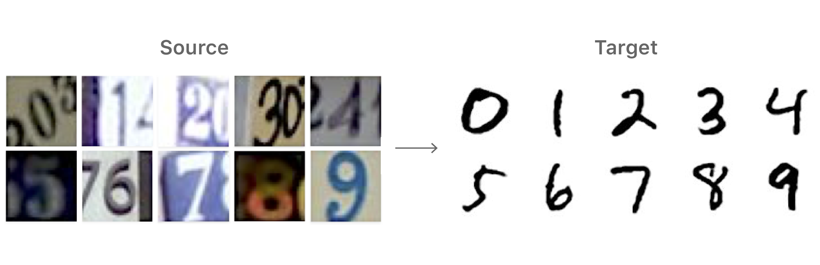
Since the task between the two datasets is to identify numbers, the expectation would be that a network trained on one dataset should perform reasonably well on the other. A typical convolutional neural network (CNN) can achieve reasonably good accuracy (98%) when trained and evaluated on the source domain (SVHN). However, the same CNN model may perform poorly (67.1% accuracy) when evaluated on the target domain (MNIST), despite the general notion that the target set is considered a less complicated task. The performance gap generally comes from the distinct distributions between the two domains. The images from the SVHN dataset contain various computer fonts, cluttered background from streets, and cropped digits near the image boundaries. Whereas the images from the MNIST dataset contain handwritten strokes and a clean background.
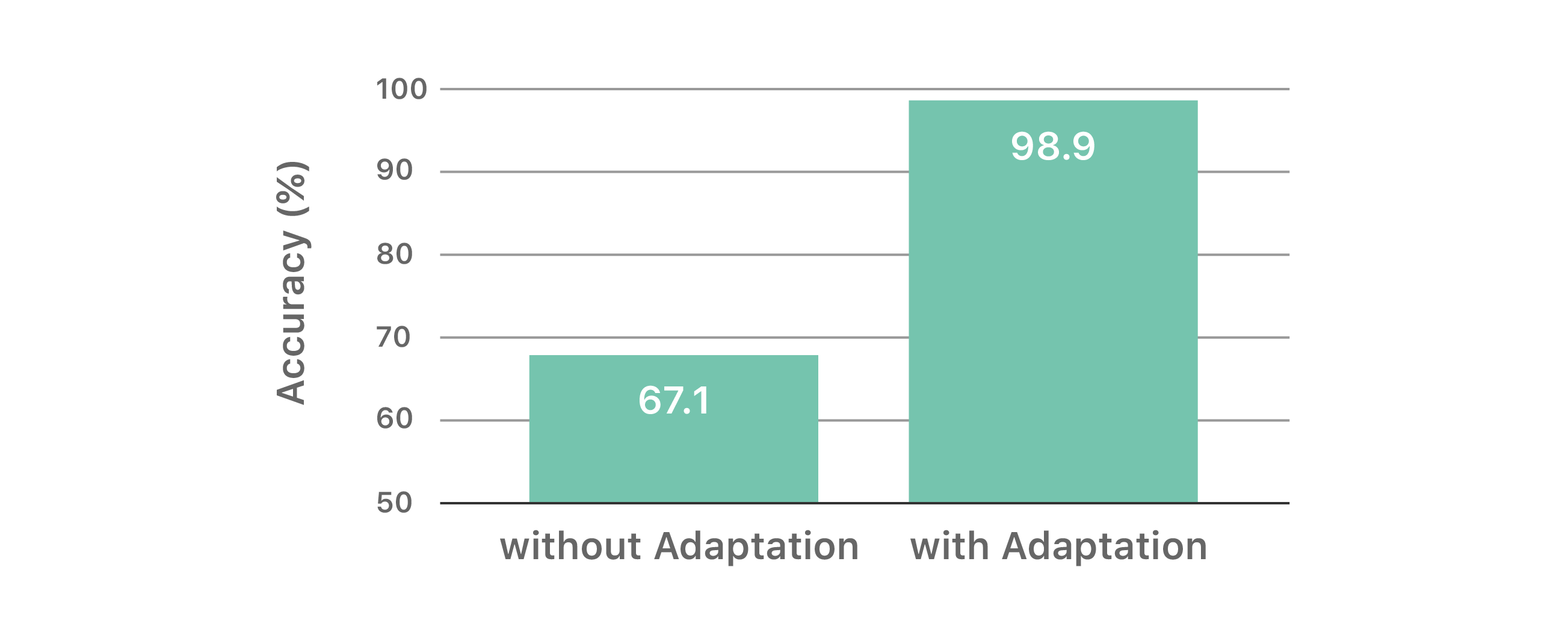
Interestingly, if we have access to part of the target set (i.e., raw images without labels) and perform some sort of domain adaptation to transfer the underlying knowledge learned from the source to target, the same CNN model can obtain immediate performance boost from 67.1% to 98.9%. This task is called the covariate shift problem, for the case where we have access to labeled data from one domain (source) and unlabeled data from another domain (target). The setup is commonly called unsupervised domain adaptation. Figure 2 summarizes the performance of the CNN model trained on the source set SVHN and evaluated on the target set MNIST with and without such unsupervised domain adaptation.
Unsupervised domain adaptation is an especially attractive alternative when the ground truth labels cannot be obtained easily for the task of interest. Unlike an image classification task, obtaining the ground truth label for each pixel in an image for a semantic segmentation task requires significant human labor. For some cases it is more difficult to obtain accurate ground truth, such as 3D bounding boxes for 3D object detection from a single image. A more feasible approach is to generate synthetic data with precise ground truths and then adapt the underlying domain knowledge to real-world data.
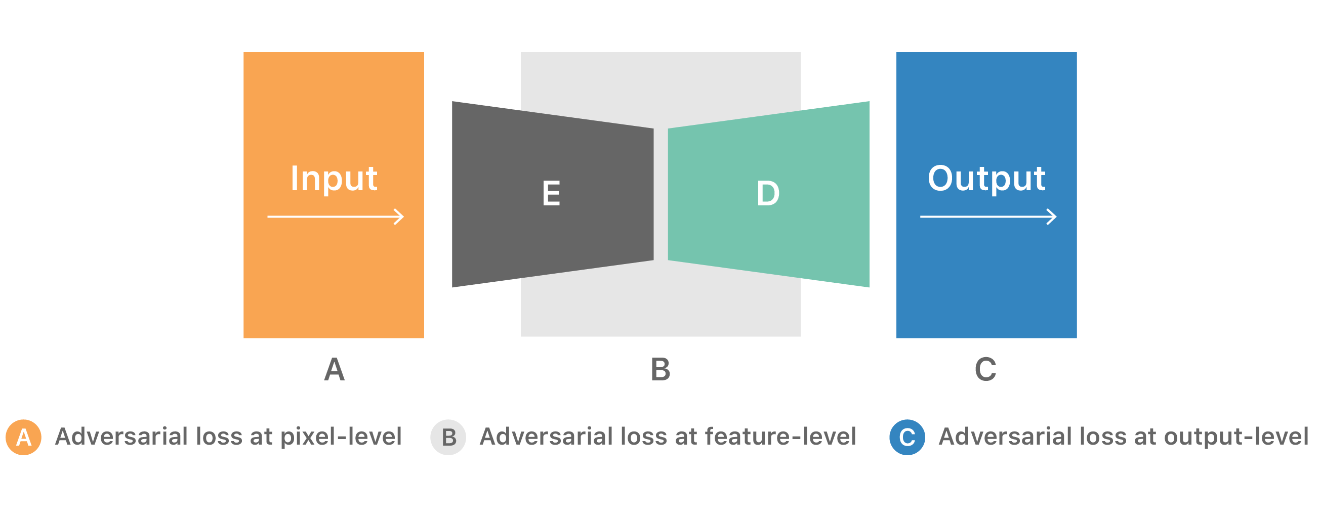
Most of the work done in this field has focused on establishing a direct alignment between the feature distribution of source and target domains. Such alignment involves minimizing some distance measure of the feature distribution learned by the models [3, 4, 5]. More sophisticated methods use adversarial training [6] to further improve the quality of alignment between distributions by adapting representations at pixel-level (as in image-to-image translation), feature-level, or output-level across domains:
However, these methods try to align distributions without the notion of the task-specific decision boundary. For example, consider the case of a semantic segmentation task of distinguishing people and roads in an urban street scene. An adversarial learning-based method for domain adaptation at pixel-level would try to translate/synthesize input images from one domain to the other, bringing the input distributions closer. The adversarial network might work very hard to synthesize photo-realistic road pixels in the new input image. Though at some point the classifier can recognize road pixels effectively and in fact requires more work to be done for the person pixels. Without knowing the current state of the task-specific decision boundary, adversarial networks might continue the effort to perfect the road pixel synthesis and therefore optimize towards an ineffective direction. Hence, it is important to preserve a notion of decision boundaries during distribution alignment.
A recent advancement that moves beyond the direction of plain distribution matching was presented by Saito et al. in [7]. They propose a within-network adversarial learning-based method containing a feature generator G, and two (task-specific) classifiers C1 and C2. These classifiers exploit the decision boundary for aligning source and target samples. The framework maximizes the discrepancy between the outputs of two classifiers to detect target samples that are outside the support of the source. They then minimize that discrepancy to generate feature representations that are within the source distribution with respect to the decision boundary. Instead of relying on heuristic assumptions, this approach focuses on molding the target data distribution by optimizing for the task.
The effectiveness of the aforementioned framework [7] depends entirely on the reliability of the discrepancy loss. Researchers have shown that neural networks tend to produce sharp distributions (i.e., probabilities that are mostly close to zero or one [8]) when trained with conventional loss functions. This limits the information that can be captured by the distance measures operating on point-wise embeddings such as L1, L2, total variation distance, Kullback-Leibler divergence, Jensen-Shannon divergence, etc.

Here we focus our efforts on improving the discrepancy measure, which plays a central role in a within-network adversarial learning-based approach [7]. We propose minimizing the cost of moving the marginal distributions between the task-specific classifiers by utilizing the Wasserstein metric [9]. This approach provides a more meaningful notion of dissimilarity for probability distributions. Wasserstein distance is able to compare distribution measures that do not overlap [10] as illustrated in Figure 4 and [11].
Computing the Wasserstein discrepancy between the classifiers’ logits requires obtaining the optimal transport coupling by solving a linear programming problem [12]. Although various optimization approaches have been proposed in the past [13], it is unclear how to directly optimize the networks efficiently over this distance measure in an end-to-end trainable fashion.
Fortunately, the Wasserstein distance for 1-D distributions has a close-form solution [14]. Therefore, we define the Sliced Wasserstein Discrepancy (SWD): a 1-D variational formulation of the Wasserstein distance between the outputs p1 and p2 of the classifiers along their radial projections. These projections are implemented as a matrix multiplication with a set of random parameters sampled from a unit sphere. This process enables the original Wasserstein distance to be effectively approximated with sufficient 1-D projections [15].
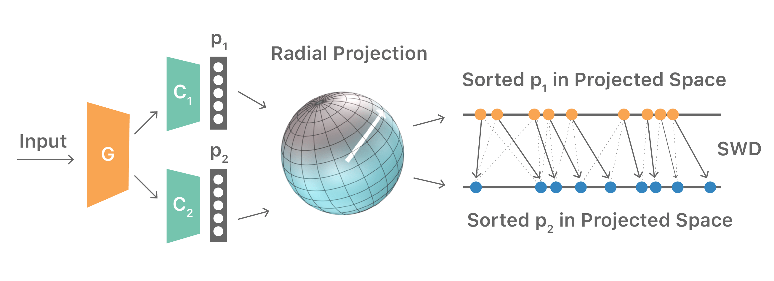
Figure 5 illustrates the SWD computation. The training procedure for the overall system pipeline can be summarized as follows:
Given a labeled source set, an unlabeled target set, and a randomly initialized feature generator G and classifiers C1, C2.
The proposed SWD integrated with within-network adversarial training effectively aligns the source and target distributions. It utilizes the task-specific decision boundaries and incorporates the Wasserstein discrepancy, which has a well-behaved energy landscape for stochastic gradient descent training.
We first demonstrate the proposed method on the Intertwining Moons 2D dataset [16]. The learned decision boundaries are shown in Figure 6 below. For the source samples, we generate an upper moon (blue points) and a lower moon (red points), labeled 0 and 1, respectively. To establish a domain shift, we generate the target samples from the source distribution by rotation and translation (green points).
After convergence (10k iteration), the source only model (Figure 6, left) classifies the source samples perfectly but does not translate well to the target samples in the bottom left and top right regions. The MCD approach [7] (Figure 6, middle) is able to adapt its decision boundary correctly in the bottom left region but not the top right region. The proposed SWD method (Figure 6, right) adapts to the target samples nicely and draws a correct decision boundary in all regions.
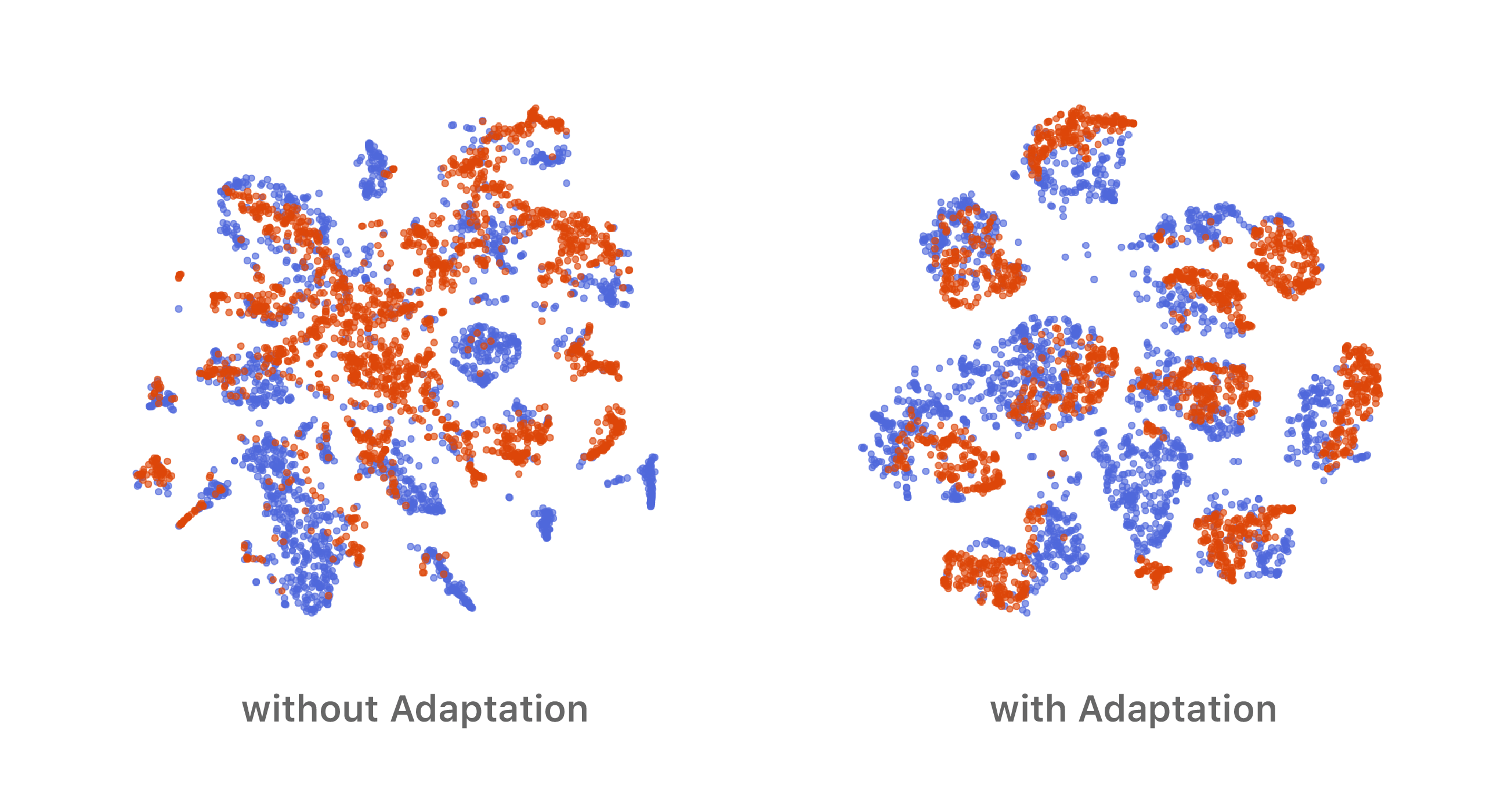
Now, let’s revisit the pilot experiment we mentioned in the beginning. We use the SVHN dataset as the source set and the MNIST dataset as the target set. We visualize the learned features in Figure 7. Our method generates much more discriminative feature representations compared to the model trained without adaptation.
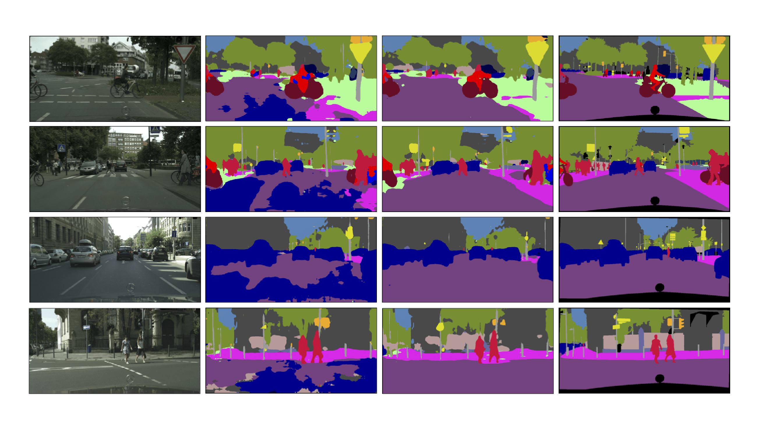
We apply the SWD to perform domain adaptation for a semantic segmentation task. In this experiment, we use three benchmark datasets: GTA5 [17], Synthia [18], and Cityscapes [19]. All three datasets contain dense pixel-level semantic annotations, which have the same class categories. During training, the synthetic GTA5 or Synthia datasets are used as the source domain and real-world Cityscapes dataset is used as the target domain. We show quantitative and qualitative results of adapting to Cityscapes in Table 1 and Figure 8, respectively. We can see clear improvements from models trained on source domain only to models trained with the proposed SWD method.
| Setting | TA5 to Cityscapes | Synthia to Cityscapes |
|---|---|---|
| No adaptation | 36.6 | 38.6 |
| SWD adaptation (ours) | 44.5 | 48.1 |
This method of unsupervised domain adaptation helps improve the performance of machine learning models in the presence of a domain shift. It enables training of models that are performant in diverse scenarios, by lowering the cost of data capture and annotation required to excel in areas where ground truth data is scarce or hard to collect. The technique can enable personalized machine learning by on-device adaptation of models for enhanced user experiences. For more details on the method described in this article, see our CVPR 2019 paper “Sliced Wasserstein Discrepancy for Unsupervised Domain Adaptation” [20] and sample source code here.
[1] Y. Netzer, T. Wang, A. Coates, A. Bissacco, B. Wu, and A. Y. Ng. Reading digits in natural images with unsupervised feature learning. In NIPS workshop, 2011.
[2] Y. LeCun, L. Bottou, Y. Bengio, and P. Haffner. Gradient-based learning applied to document recognitio. Proceedings of the IEEE, 1998.
[3] K. Saenko, B. Kulis, M. Fritz, and T. Darrell. Adapting visual category models to new domains. In ECCV, 2010.
[4] Y. Ganin and V. Lempitsky. Unsupervised domain adaptation by backpropagation. In ICML, 2014.
[5] M. Long, Y. Cao, J. Wang, and M. I. Jordan. Learning transferable features with deep adaptation networks. In ICML, 2015.
[6] I. Goodfellow, J. Pouget-Abadie, M. Mirza, B. Xu, D. Warde-Farley, S. Ozair, A. Courville, and Y. Bengio. Generative adversarial nets. In NIPS, 2014.
[7] K. Saito, K. Watanabe, Y. Ushiku, and T. Harada. Maximum classifier discrepancy for unsupervised domain adaptation. In CVPR, 2018.
[8] G Pereyra, G Tucker, J Chorowski, L Kaiser, and G Hinton. Regularizing Neural Networks by Penalizing Confident Output Distributions. CoRR abs/1701.06548, 2017.
[9] C. Villani. Optimal transport, old and new. Springer-Verlag, 2009.
[10] M. Arjovsky, S. Chintala, and L. Bottou. Wasserstein generative adversarial networks. In ICML, 2017.
[11] http://www.stat.cmu.edu/~larry/=sml/Opt.pdf
[12] L. Kantorovitch. On the translocation of masses. Management Science, 1958.
[13] M. Cuturi. Sinkhorn distances: Lightspeed computation of optimal transport. In NIPS, 2013.
[14] J Rabin, G Peyré, J Delon, and M Bernot. Wasserstein barycenter and its application to texture mixing. In SSVM, 2011.
[15] N Bonnotte. Unidimensional and evolution methods for optimal transportation. Doctoral dissertation, Paris 11, 2013.
[16] F Pedregosa et al. Scikit-learn: Machine learning in python. JMLR, 2011.
[17] S Richter, V Vineet, S Roth, and V Koltun. Playing for data: Ground truth from computer games. In ECCV, 2016.
[18] G Ros, L Sellart, J Materzynska, D Vazquez, and A Lopez. The synthia dataset: A large collection of synthetic images for semantic segmentation of urban scenes. In CVPR, 2016.
[19] M Cordts, M Omran, S Ramos, T Rehfeld, M Enzweiler, R Benenson, U Franke, S Roth, and B Schiele. The cityscapes dataset for semantic urban scene understanding. In CVPR, 2016.
[20] CY Lee, T Batra, MH Baig, and D Ulbricht. Sliced Wasserstein Discrepancy for Unsupervised Domain Adaptation. In CVPR, 2019.
Corpus Synthesis for Zero-shot ASR Domain Adaptation using Large Language Models
March 14, 2024research area Speech and Natural Language Processingconference ICASSP
While Automatic Speech Recognition (ASR) systems are widely used in many real-world applications, they often do not generalize well to new domains and need to be finetuned on data from these domains. However, target-domain data is usually not readily available in many scenarios. In this paper, we propose a new strategy for adapting ASR models to new target domains without any text or speech from those domains. To accomplish this, we propose a…
Sliced Wasserstein Discrepancy for Unsupervised Domain Adaptation
March 10, 2019research area Methods and Algorithmsconference CVPR
In this work, we connect two distinct concepts for unsupervised domain adaptation: feature distribution alignment between domains by utilizing the task-specific decision boundary and the Wasserstein metric. Our proposed sliced Wasserstein discrepancy (SWD) is designed to capture the natural notion of dissimilarity between the outputs of task-specific classifiers. It provides a geometrically meaningful guidance to detect target samples that are…

Our research in machine learning breaks new ground every day.