ParaRNN: Large-Scale Nonlinear RNNs, Trainable in Parallel

Recurrent Neural Networks (RNNs) are naturally suited to efficient inference, requiring far less memory and compute than attention-based architectures, but the sequential nature of their computation has historically made it impractical to scale up RNNs to billions of parameters. A new advancement from Apple researchers makes RNN training dramatically more efficient — enabling large-scale training for the first time and widening the set of architecture choices available to practitioners in designing LLMs, particularly for resource-constrained deployment.

In ParaRNN: Unlocking Parallel Training of Nonlinear RNNs for Large Language Models, a new paper accepted to ICLR 2026 as an Oral, Apple researchers share a new framework for parallelized RNN training that achieves a 665× speedup over the traditional sequential approach (see Figure 1). This efficiency gain enables the training of the first 7-billion-parameter classical RNNs that can achieve language modeling performance competitive with transformers (see Figure 2).

To accelerate research in efficient sequence modeling and enable researchers and practitioners to explore new nonlinear RNN models at scale, the ParaRNN codebase has been released as an open-source framework for automatic training-parallelization of nonlinear RNNs.

Speedup from Parallel RNN Training

ParaGRUParaLSTM

Performance of Large-Scale Classic RNNs

1B2.9B7B

Why Recurrent Models Still Matter

The computational cost of the attention mechanism in a transformer grows quadratically with sequence length, whereas the computation required for a single forward pass through an RNN is the same regardless of how much context came before. This enables constant-time token generation during inference, making them particularly attractive for efficient deployment.

But there’s a catch: this efficiency advantage only applies at inference time. Unlike transformers, RNN training can’t be parallelized along the sequence length.

The Training Bottleneck

The very property that makes RNN efficient at inference — their sequential, recurrent structure — becomes a fundamental bottleneck during training. Unlike the attention mechanism, which can process all tokens in a sequence simultaneously, an RNN application must be unrolled step-by-step, as illustrated in Figure 3.

Fundamental trade-off between RNNs and Attention

A Compromise for Parallelizability: Linearity

Modern recurrent architectures have leveraged a clever workaround to enable sequence parallelization: simplifying the recurrence relationship to be purely linear in the hidden state. Selective state space models (SSMs) like Mamba use a recurrence in the form:

$$\text{SSMs: } h_{l} = A_l h_{l-1} + B_l x_l,$$

while classical RNNs include nonlinearities:

$$\text{RNNs: } h_l = \sigma_l(h_{l-1}, x_l).$$

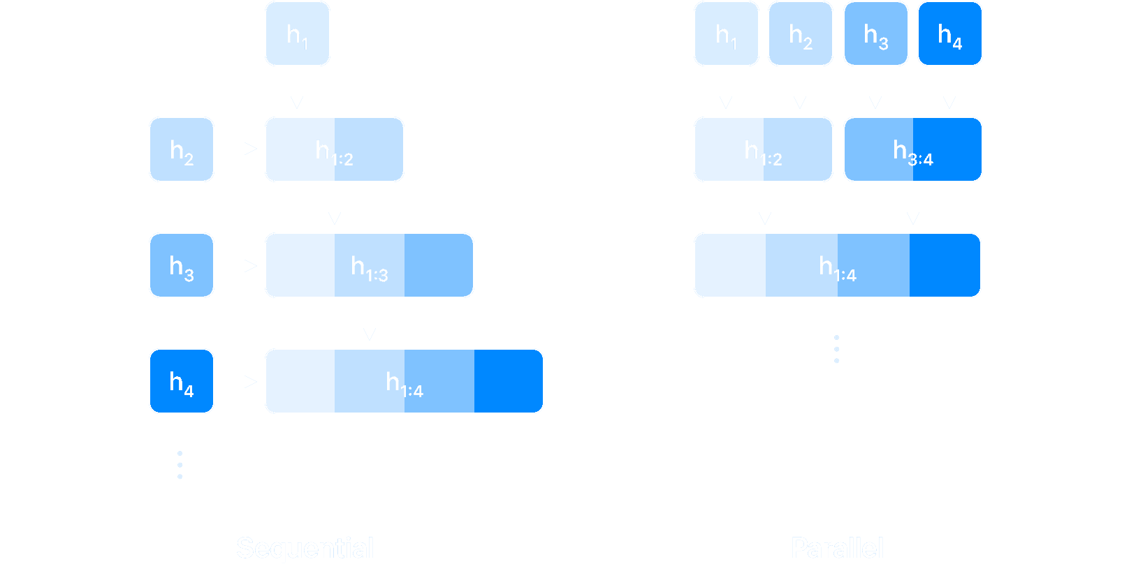
Linearity enables parallelization because linear operations are associative, meaning the order in which you combine them doesn’t affect the final result, just like $(2+3)+4=2+(3+4)$. This mathematical property allows us to use parallel reduction algorithms (also known as parallel scan) to compute the entire sequence of hidden states simultaneously. The intuition is the same behind the parallel computation of a cumulative sum: rather than sequentially adding new terms (starting with $h_1$, add $h_2$, then $h_3$ …), one can compute partial results in parallel (add $h_1$, and $h_2$, at the same time as $h_3$ and $h_4$ and $h_5$ and $h_6$, …) and combine them in a tree-like structure, as illustrated in Figure 4. This approach transforms the SSM application from $\mathcal{O}(L)$ sequential steps to $\mathcal{O}(\log_2L)$ parallel steps, which makes for a dramatic speedup for long sequences: doubling the sequence length only requires one extra step, instead of double the amount.

A Compromise for Parallelizability: Linearity

Linearity, however, comes with its own set of limitations: the types of hidden state evolutions that can be modeled by a linear system is reduced in its variety, which has a direct impact on the overall expressivity of the RNN model. The question then becomes: must we sacrifice expressivity for speed, or can we have both?

Parallel Training of Nonlinear RNNs: Newton Strikes Again

The key insight is that we can have the best of both worlds, by adapting Newton’s method — a classic numerical technique for solving nonlinear equations. Rather than tackling the complex system directly, Newton’s method works by iteratively building and solving an approximation (in the form of a more tractable linear system) which is used to progressively refine the solution to the target nonlinear one.

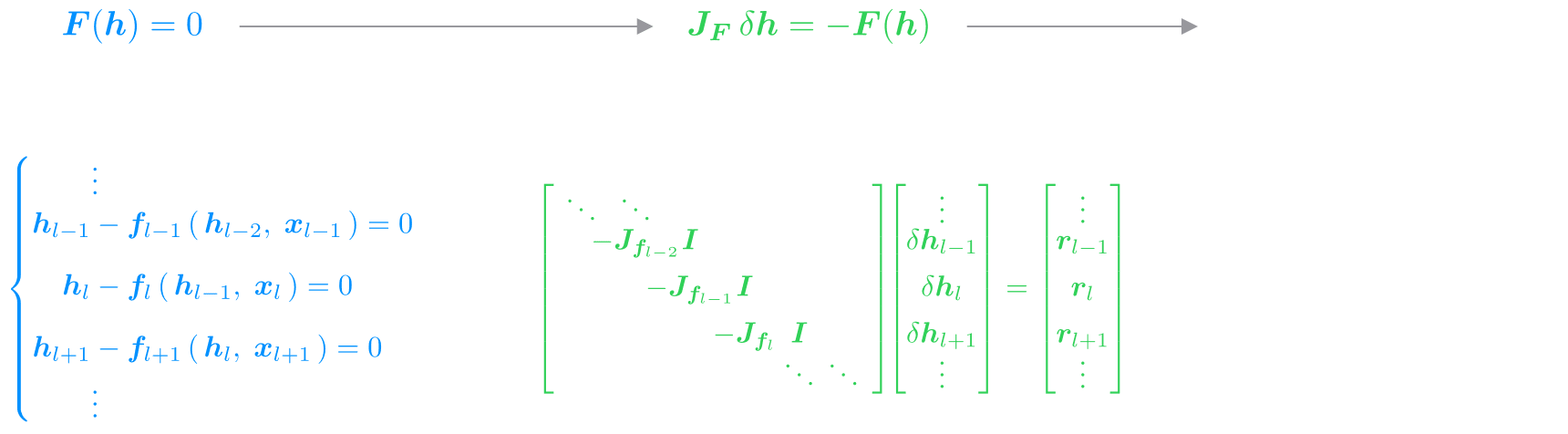
In Figure 5 we illustrate how we can apply this to our scenario. Instead of thinking of the RNN as a chain of sequential steps, we reframe the entire sequence as a single system of equations, where the hidden states across all steps are unknowns to solve for simultaneously. Newton’s method solves this system iteratively, approximating the nonlinearities with a linearization given by their local derivatives (i.e., their Jacobians). This is where the magic happens: the linearized RNN system has exactly the same form as a linear SSM, with the Jacobians playing the role of the state matrices $A_l$​. We are effectively turning the solution of a nonlinear RNN into the iterative solution of linear SSMs, each of which can be efficiently solved in parallel.

While this approach introduces some overhead with respect to computing the RNN application sequentially, if the Newton iterations converge quickly enough (which we empirically observed for well-designed RNN models), we can effectively recover the full nonlinear RNN behavior in a fraction of the time, thanks to parallelization.

Newton’s Method Applied

In our experiments, we apply this methodology to adaptations of two classical RNNs: the GRU and LSTM cells, and achieve convergence consistently with just three iterations. In other words, with three carefully designed, parallel SSM applications, we can recover the same hidden state evolution as with the sequential application of a nonlinear RNN — dramatically reducing wall-clock time at training.

Scaling Up: Structured Jacobians and Optimized Kernels

While the ParaRNN framework can in principle be applied to any RNN, some careful engineering is still required to make it practical for large-scale training. The parallel reduction algorithm at the heart of the method needs to efficiently assemble, store, and multiply together the Jacobian matrices arising from the linearization. For generic RNNs, these Jacobians are dense, which makes their storage grow quadratically and their multiplication cubically with hidden state size — a cost intractable for large-scale models.

We address this following the design principles from modern SSMs like Mamba, and introduce the ParaGRU and ParaLSTM cells: adaptations of the classical GRU and LSTM cells that yield structured Jacobians. In particular, we simplify the matrices in the cells’ definition to only have nonzero elements in their main diagonal. This ensures that their Jacobians are also diagonal (for ParaGRU) and block-diagonal (for ParaLSTM), as outlined in Figure 6.

General: denseStructured: (block) diagonal

To get the best speedups, we then implement custom CUDA kernels to perform efficient parallel reduction of Jacobians presenting these structures. In the design of our kernels, we make sure to closely follow the GPU memory hierarchy to keep the data as local as possible. As a result, our fully-fused implementation handles Newton iterations, system assembly, and parallel reduction in a single kernel, achieving remarkable speedups over Mamba, In Figure 7 we provide timing results for the three implementations we provide to apply our ParaRNN cells in parallel: in pure PyTorch, in PyTorch with CUDA-accelerated reduction, and fully-fused in CUDA.

Forward Pass through ParaGRU and ParaLSTM Cells

ParaGRUParaLSTM

Results

To validate the effectiveness of the ParaRNN framework in enabling practical training of nonlinear RNNs at scale, we trained models ranging from 400M to 7B parameters on language modelling tasks. Our goal is to test how classical RNNs can perform as LLMs, once large-scale training becomes feasible via parallelization.

Classical RNNs as Large Language Models

The results show that even classical RNNs make for competitive LLMs when trained at the 7B scale. Both in terms of sheer perplexity and downstream task performance (see Table 1), ParaGRU and ParaLSTM achieve scores comparable to transformers and state-of-the-art SSMs.

	Model	#params	↓ PPL	↑ Arc-C (25)   (3)		↑ HSwag (10)   (0)		↑ OBQA (10)   (0)		↑ WinoG (5)   (0)		↑ PiQA (0)	↑ MMLU (0)
	Mamba2	6.96B	8.62	40.02	39.59	69.78	69.68	42.20	42.20	65.19	63.77	76.66	26.61
	ParaLSTM	6.76B	9.16	37.46	36.52	62.47	62.85	42.20	38.80	57.70	59.12	75.19	25.31
	ParaGRU	6.76B	9.19	39.68	36.77	65.85	65.75	42.20	40.40	61.40	59.83	76.66	25.29
	Transformer	6.89B	9.55	34.30	33.36	62.98	62.20	40.00	37.20	61.48	60.85	74.97	23.12

Faster Throughput

The real advantage of recurrent models shines at inference time, as shown in Figure 8. The constant-time token generation of RNNs means maintaining high throughput regardless of context length, making them an appealing choice for applications where achieving fast generation is paramount.

Model Throughput

Nonlinearities Matter

Moreover, the ability to include nonlinearities in the recurrence step definition dramatically boosts performance on synthetic tasks requiring state tracking and retrieval capabilities. These are useful to test the model’s ability to maintain and update meaningful information in its internal state, and to store and recover relevant information when needed. The improved performance outlined in Table 2 indicates that nonlinear RNNs provide superior expressivity over linear ones, and are worth considering to design more powerful models.

	Model	MQAR	𝑘-hop	Parity
	Transformer	100%	78%	53%
	Mamba2	100%	98%	51%
	ParaGRU	100%	100%	100%
	ParaLSTM	100%	100%	100%

Ultimately, our experiments show that scalability was the missing piece in the RNN puzzle all along. At billion scale, they perform as well as modern language models, and boast superior expressivity and faster throughput to boot. These results open the door to reconsidering nonlinear recurrence in modern sequence modelling: the nonlinearity vs training efficiency trade-off isn’t fundamental — it was just a consequence of computational limitations, which we can now overcome.

Build Your Own Parallel RNN

To accelerate progress and enable further exploration nonlinear RNN models at scale, the ParaRNN codebase has been released as an open-source framework. Researchers and practitioners can just focus on designing the RNN cell — the framework takes care of everything else.

Three Lines to Parallel Training

To define a custom cell in ParaRNN, just implement its recurrence step:

class MyRNNCell( BaseRNNCell ):
    def recurrence_step( self, h, x, system_parameters ):
        h_new = ... # \sigma( h, x; params )
        return h_new

The framework automatically handles Newton’s method application, Jacobian assembly, parallel reduction routines, and optimizations for structured Jacobians.

Three Performance Tiers

• Pure PyTorch: For prototyping. Uses automatic differentiation and works for any RNN, but is not optimized for scale
• CUDA-Accelerated: For generic cells with (block-)diagonal Jacobians. Uses custom kernels for parallel reduction
• Fully-Fused: Single-kernel implementation fusing the whole Newton routine. Requires CUDA implementation of recurrence step

The modular design makes it easy to experiment with custom cells, Jacobian structures, and solver configurations—it suffices to inherit from the available base classes and implement the specific reduction operations.

RNNs are Back

RNN application is not inherently sequential anymore. For the first time, classical RNNs can be trained at the scale of billions of parameters with training times and performance matching modern architectures — unlocking the inference efficiency and expressivity advantages that made recurrence appealing in the first place.

ParaRNN opens the door to exploring nonlinear recurrence at scale: experimenting with novel architectures and pushing the boundaries of what’s possible with recurrent models is now easier than ever. Nonlinear RNNs are back and ready to scale.