content type highlightpublished July 7, 2017
Improving the Realism of Synthetic Images
Improving the Realism of Synthetic Images
Most successful examples of neural nets today are trained with supervision. However, to achieve high accuracy, the training sets need to be large, diverse, and accurately annotated, which is costly. An alternative to labelling huge amounts of data is to use synthetic images from a simulator. This is cheap as there is no labeling cost, but the synthetic images may not be realistic enough, resulting in poor generalization on real test images. To help close this performance gap, we’ve developed a method for refining synthetic images to make them look more realistic. We show that training models on these refined images leads to significant improvements in accuracy on various machine learning tasks.
Training machine learning models on standard synthetic images is problematic as the images may not be realistic enough, leading the model to learn details present only in synthetic images and failing to generalize well on real images. One approach to bridge this gap between synthetic and real images would be to improve the simulator which is often expensive and difficult, and even the best rendering algorithm may still fail to model all the details present in the real images. This lack of realism may cause models to overfit to ‘unrealistic’ details in the synthetic images. Instead of modeling all the details in the simulator, could we learn them from data? To this end, we developed a method for refining synthetic images to make them look more realistic (Figure 1).
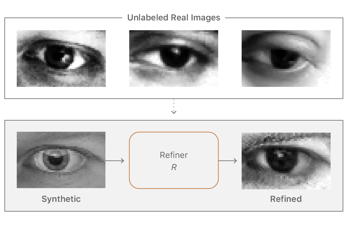
The goal of ‘improving realism’ is to make the images look as realistic as possible to improve the test accuracy. This means we want to preserve annotation information for training of machine learning models. For example, the gaze direction in Figure 1 should be preserved, as well as not generate any artifacts, as machine learning models could learn to overfit to them. We learn a deep neural network, which we call ‘refiner network’, that processes synthetic images to improve their realism.
To learn such a refiner network, we need some real images. One option would be to require pairs of real and synthetic images with pixel-wise correspondence, or real images with annotations—e.g. the gaze information in the case of eyes. This is arguably an easier problem, but such data is very difficult to collect. To create pixel-wise correspondence, we need to either render a synthetic image that corresponds to a given real image, or capture a real image that matches a rendered synthetic image. Could we instead learn this mapping without pixel-wise correspondence, or any labels for the real images? If so, we could just generate a bunch of synthetic images, capture real images of eyes, and without labeling any real images at all, learn this mapping—making the method cheap and easy to apply in practice.
To learn our refiner network in an unsupervised manner, we utilize an auxiliary discriminator network that classifies the real and the refined (or fake) images into two classes. The refiner network tries to fool this discriminator network into thinking the refined images are the real ones. Both the networks train alternately, and training stops when the discriminator cannot distinguish the real images from the fake ones. The idea of using an adversarial discriminator network is similar to the GANs (Generative Adversarial Networks [1]) approach that maps a random vector to an image such that the generated image is indistinguishable from the real ones. Our goal is to train a refiner network—a generator—that maps a synthetic image to a realistic image. Figure 2 shows an overview of the method.
In addition to generating realistic images, the refiner network should preserve the annotation information of the simulator. For example, for gaze estimation the learned transformation should not change the gaze direction. This restriction is an essential ingredient to enable training a machine learning model that uses the refined images with the simulator’s annotations. To preserve the annotations of synthetic images, we complement the adversarial loss with a self-regularization L1 loss that penalizes large changes between the synthetic and refined images.
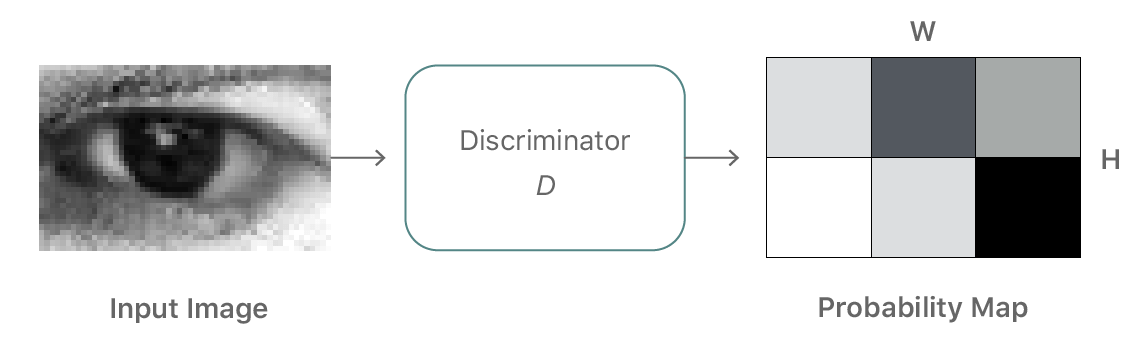
Another key requirement for the refiner network is that it should learn to model the real image characteristics without introducing any artifacts. When we train a single strong discriminator network, the refiner network tends to over-emphasize certain image features to fool the current discriminator network, leading to drifting and producing artifacts. A key observation is that any local patch sampled from the refined image should have similar statistics to a real image patch. Therefore, rather than defining a global discriminator network, we can define a discriminator network that classifies all local image patches separately (Figure 3). This division not only limits the receptive field, and hence the capacity of the discriminator network, but also provides many samples per image for learning the discriminator network. The refiner network is also improved by having multiple ‘realism loss’ values per image.
The generator can fool the discriminator either with samples from a novel distribution or the target (real data) distribution. Generating from a novel distribution fools the discriminator only until the discriminator learns that novel distribution. The more useful way the generator can fool the discriminator is by generating from the target distribution.
Given these two ways of evolving, the easiest is usually to generate a novel output, which is what we observed when training the current generator and discriminator against each other. A simplified illustration of this unproductive sequence is shown in the left-hand side of Figure 4. The generator and discriminator distributions are shown in yellow and blue respectively.
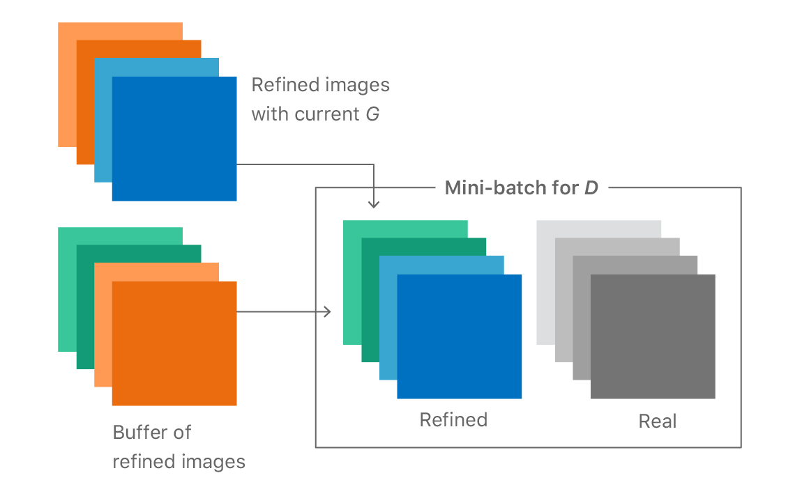
By introducing a history which stores generator samples from previous generations (right-hand of Figure 4), the discriminator is less likely to forget the part of the space about which it has already learned. The more powerful discriminator helps the generator to move toward the target distribution faster. The illustration is a simplification and neglects to show that the distributions are complex and often disconnected regions. In practice however, a simple random replacement buffer captures enough diversity from previous generator distributions to prevent repetition by strengthening the discriminator. Our notion is that any refined image generated by the refiner network at any time during the entire training procedure is really a ‘fake’ image for the discriminator. We found that by constructing a mini-batch for D with half the samples from the history buffer and the other half from the current generator’s output (as shown in Figure 5) we can improve training.
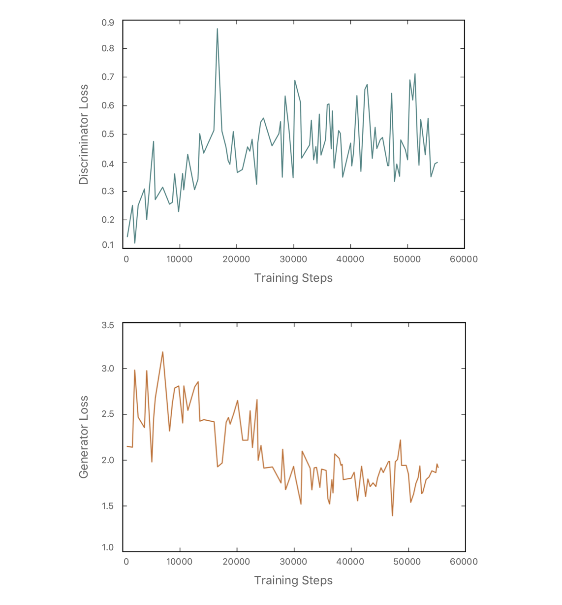
We first train the refiner network with only self-regularization loss, and introduce the adversarial loss after the refiner network starts producing blurry versions of the input synthetic images. Figure 6 shows the output of refiner network at various steps of training. In the beginning, it outputs a blurry image that becomes more and more realistic as training progresses. Figure 7 visualizes the discriminator and generator losses at different training iterations. Note that the discriminator loss is low in the beginning—meaning it can easily tell the difference between real and refined. Slowly, the discriminator loss increases and the generator loss decreases as training progress, generating more real images.
When the synthetic and real images have significant shift in the distribution, a pixel-wise L1 difference may be restrictive. In such cases, we can replace the identity map with an alternative feature transform, putting a self-regularizer on a feature space. These could be hand-tuned features, or learnt features such as a mid layer from VGGnet. For example, for color image refinement, the mean of RGB channels can generate realistic color images such as in Figure 8.
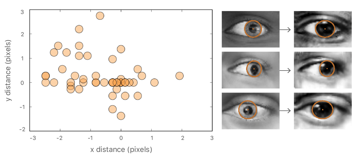
To verify that the labels do not change significantly, we manually drew ellipses on the synthetic and refined images, and computed the difference between their centers. In Figure 9, we show a scatter plot of 50 such center differences. The absolute difference between the estimated pupil center of synthetic and corresponding refined image is quite small: 1.1 +/- 0.8px (eye width = 55px).
First we initialized G only with the self-regularization loss so that it can start producing blurry version of the synthetic input. Typically it took 500-2,000 steps of G (without training D).
We used different number of steps for the generator and discriminator in each training iteration. For hand-pose estimation using depth, we used 2 steps of G for each D step, and for eye gaze estimation experiment we ended up using 50 steps of G for each D step. We found the discriminator to converge more quickly compared to the generator, partly because of the batch-norm in the discriminator. So, we fixed the #D steps to 1, and started varying #G steps starting from a small number, slowly increasing it depending on the discriminator loss values.
We found it helpful to keep learning rate very small (~0.0001) and train for a long time. This approach worked probably because it keeps both the generator or the discriminator from making sudden shifts which would leave the other behind. We found it difficult to stop the training by visualizing the training loss. Instead, we saved training images as training progresses, and stopped training when the refined images looked visually similar to real images.
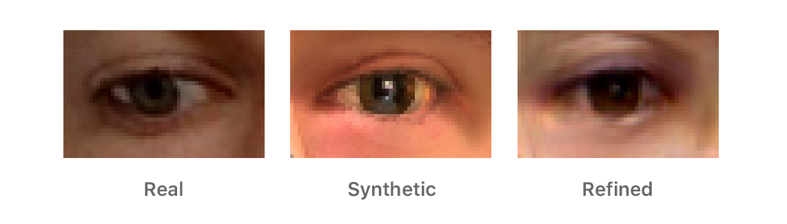
To evaluate the visual quality of the refined images, we designed a simple user study where subjects were asked to classify images as real or refined synthetic. The subjects found it very difficult to tell the difference between the real and refined images. In our aggregate analysis, 10 subjects chose the correct label 517 times out of 1000 trials, meaning they were not able to reliably distinguish real images from refined synthetic ones. In contrast, when testing on original synthetic images vs real images, we showed 10 real and 10 synthetic images per subject, and the subjects chose correctly 162 times out of 200 trials. In Figure 10 we show some example synthetic and corresponding refined images.
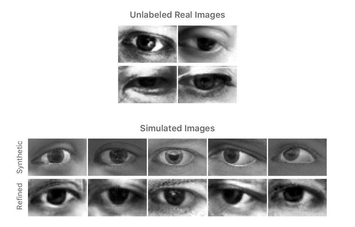
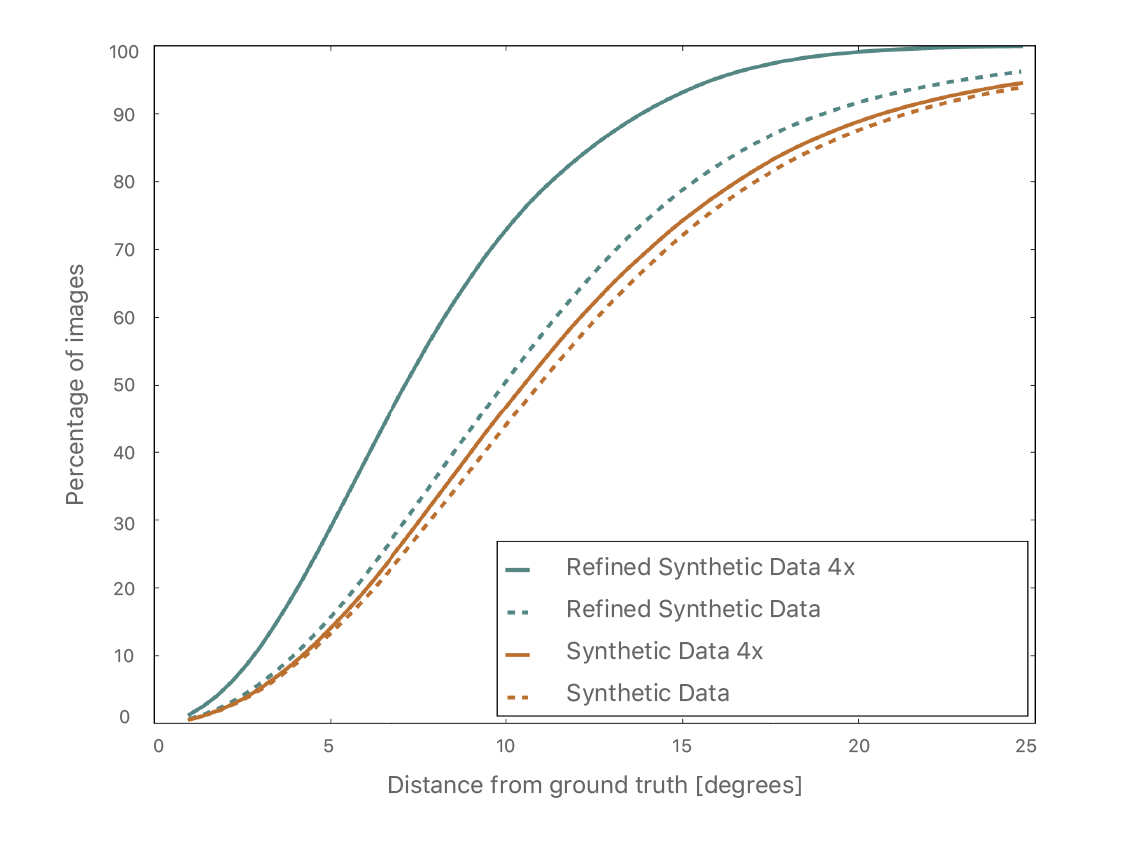
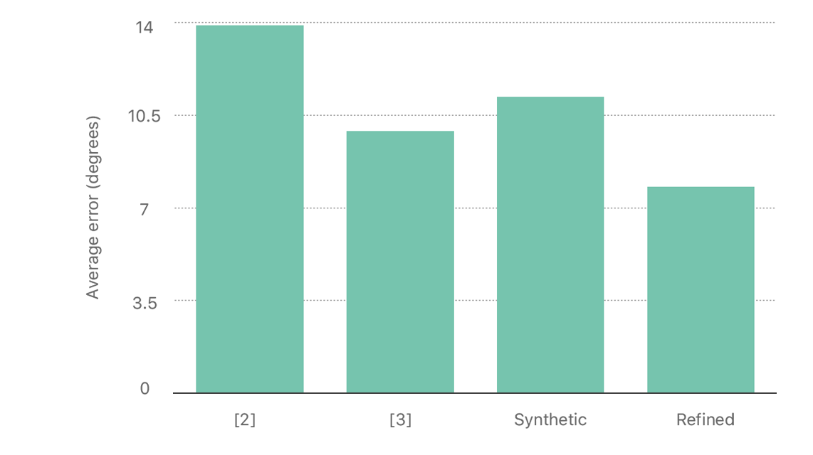
Figure 11 shows the improvement using refined data, compared to training with original synthetic data. Two things to note from this figure: (1) Training with refined images is better than training with original synthetic images, and (2) using more synthetic data further improves performance. In Figure 12, we compare the gaze estimation error with other state-of-the-art methods, and show that improving the realism significantly helps the model generalize on real test data.
Recently there has been a lot of interest in domain adaptation using adversarial training. The image-to-image translation [4] paper by Isola et al. describe a method that learns to change an image from one domain to another, but it needs pixel-wise correspondences. The unpaired image-to-image translation paper [5] discussing relaxing the requirement of pixel-wise correspondence, and follows our strategy of using the generator history to improve the discriminator. The unsupervised image-to-image translation network [6] uses a combination of a GAN and variational auto-encoder to learn the mapping between source and target domains. Costa et al. [7] use ideas from our work to learn to generate images of the eye fundus. Sela et al. [8] use a similar self-regularization approach for facial geometry reconstruction. Lee et al. [9] learn to synthesize an image from key local patches using a discriminator on patches. For more details on the work we describe in this article, see our CVPR paper “Learning from Simulated and Unsupervised Images through Adversarial Training” [10].
[1] I. J. Goodfellow, J. Pouget-Abadie, M. Mirza, B. Xu, D. Warde-Farley, S. Ozair, A. Courville, and Y. Bengio, Generative Adversarial Nets. Proceedings Neural Information Processing Systems Conference, 2014.
[2] X. Zhang, Y. Sugano, M. Fritz, and A. Bulling, Appearance-based Gaze Estimation in the Wild. Proceedings Computer Vision Pattern Recognition Conference, 2015.
[3] E. Wood, T. Baltrušaitis, L.-P. Morency, P. Robinson, and A. Bulling, Learning an Appearance-based Gaze Estimator from One Million Synthesised Images. Proceedings ACM Symposium on Eye Tracking Research & Applications, 2016.
[4] P. Isola, J.-Y. Zhu, T. Zhou, and A. A. Efros, Image-to-Image Translation with Conditional Adversarial Networks. ArXiv, 2016.
[5] J.-Y. Zhu, T. Park, P. Isola, and A. A. Efros, Unpaired Image-to-Image Translation using Cycle-Consistent Adversarial Networks. ArXiv, 2017.
[6] M.-Y. Liu, T. Breuel, and J. Kautz, Unsupervised Image-to-Image Translation Networks. ArXiv, 2017.
[7] P. Costa, A. Galdran, M. I. Meyer, M. D. Abràmoff, M. Niemeijer, A. M.Mendonça, and A. Campilho, Towards Adversarial Retinal Image Synthesis. ArXiv, 2017.
[8] M. Sela, E. Richardson, and R. Kimmel, Unrestricted Facial Geometry Reconstruction Using Image-to-Image Translation. ArXiv, 2017
[9] D. Lee, S.Yun, S. Choi, H. Yoo, M.-H. Yang, and S. Oh, Unsupervised Holistic Image Generation from Key Local Patches. ArXiv, 2017.
[10] A. Shrivastava, T. Pfister, O. Tuzel, J. Susskind, W. Wang, R. Webb, Learning from Simulated and Unsupervised Images through Adversarial Training. CVPR, 2017.
An On-device Deep Neural Network for Face Detection
November 16, 2017research area Computer Vision, research area Methods and Algorithms
Apple started using deep learning for face detection in iOS 10. With the release of the Vision framework, developers can now use this technology and many other computer vision algorithms in their apps. We faced significant challenges in developing the framework so that we could preserve user privacy and run efficiently on-device. This article discusses these challenges and describes the face detection algorithm.
Learning from Simulated and Unsupervised Images through Adversarial Training
July 19, 2017research area Computer Visionconference CVPR
With recent progress in graphics, it has become more tractable to train models on synthetic images, potentially avoiding the need for expensive annotations. However, learning from synthetic images may not achieve the desired performance due to a gap between synthetic and real image distributions. To reduce this gap, we propose Simulated+Unsupervised (S+U) learning, where the task is to learn a model to improve the realism of a simulator’s output…

Our research in machine learning breaks new ground every day.